Structure from Motion (SfM) Derived Digital Surface Models from a Trimble UX5 Flight using GRASS
Problem Description
Evaluation of digital surface model’s (DSMs) accuracy is an important step before conducting any sort of data analysis. For this project, GRASS was used to compare several DSMs created from the same UAS flight. Agisoft and Pix4D were used to construct the various DSMs. The data used was from a Trimble UX5 flight over the Mid Pines area off of Lake Wheeler Rd. near NCSU in September of 2015.
Analysis Procedures
These DSMs were all created using SfM over the Lake Wheeler property. The multiple DSMs allowed for comparisons of software plus comparisons of results where GCPs were used and where GCPs were not used. Differences in elevation between DSMs with GCPs and those without were calculated using raster map algebra through GRASS’s r.mapcalc module. Additionally, raster algebra was used to determine which software created a DSM with the largest bowl effect. This was done by comparing three DSMs with GCPs from Agisoft, Pix4D and Trimble Business Center. These three DSMs were them compared to two DSMs created in Agisoft and Pix4D with no GCPs.
To determine the locations of artifacts, a basic terrain analysis was done using GRASS’s r.slope.aspect module. Several GRASS GIS Addons were downloaded (r.local.relief, r.shaded.pca and r.skyview) to further visually inspect the data. Lastly, an evaluation of terrain changes between UAS flights was completed by again using map algebra.
Results
The images included below show some of the analysis and evaluations conducted on the Agisoft and Pix4D created DSMs and shows the improved accuracy of results when using GCPs. For example, the ‘bowl effect’, an artifact due to the camera lense, is minimized when GCPs are used. Figure 1 below shows the ‘bowl effect’ by comparing DSMs created in Agisoft and Pix4D.


Figure 1 Both of these show elevation differences from a GCP DSM and a non-GCP derived DSM. The image on the left are from DSMs created in Agisoft and on the left DSMs created in Pix4D.
The 3 images below are comparisons to decide what software generates the largest bowl effect. The largest differences appear between the Agisoft and Pix4D DSMs (Figure 2b). These differences appear near the edges, which could corroborate the results in Figure 1 where the Agisoft non-GCP DSM displayed a large bowl effect.


Figure 2a (left) This image is a comparison of elevation between Agisoft and Trimble. Figure 2b (middle) This image shows the differences between Agisoft and Pix4D. Figure 2c (right) This image shows the differences between the Pix4D DSM and the Trimble DSM.
The last analysis done was to calculate changes in DSMs from June to October for the Lake Wheeler Road property. The difference map is shown in Figure 3 below. The elevation difference indicates gain (positive) and loss of elevation (negative) in the months between mapping missions. A key point to note is that 11 GCPs were used in the June flight and 8 for the October flight. This may contribute to slight changes in elevation in generated DSMs. Large areas of differences are shown in the fields, which can be explained by mowing. Also, a logical change in height in the months between flights would be to trees. These changes are identified in the comparison map.
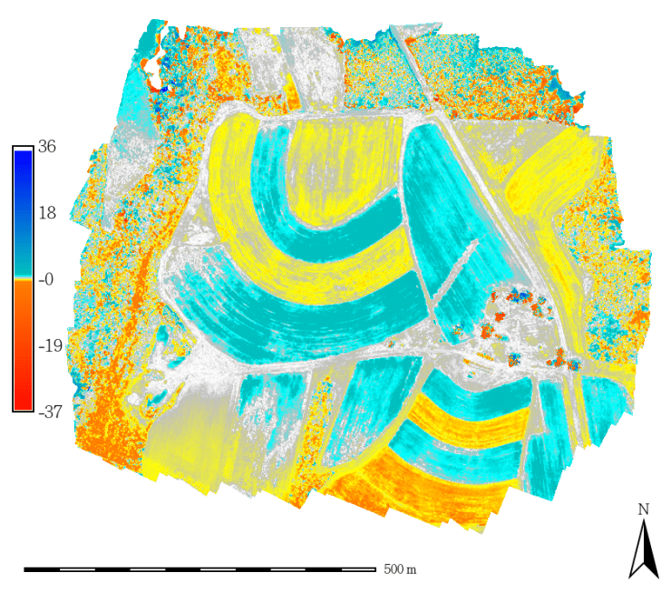
Figure 3 This image shows the differences in derived DSMs from flights in June and October of the same year.
Reflection
Using the tools and modules in GRASS enabled DSMs from different flights and derived from different software packages to be analyzed. It was also apparent that the use of GCPs during the DSM creation process is important. Differences were noted between DSMs were GCPs were used and those where GCPs were not. It is important to consider the underlying process during DSM derivation to conduct a robust analysis on the resulting DSM. Identification of artifacts is important and can be done using GRASS and similar software.
This was an enjoyable exercise and always enjoy using GRASS. It’s intuitive and using the command line allows for conceptualization of the tools that are being run. This assignment helped in the understanding that it’s important to consider how a DSM is derived. For future work, I will pay attention to if/how GCPs are used, what differences in DSMs for the same location can mean and how software can impact the resulting DSM.
________________________
Creation and Implementation of a Landslide Potential Index (LPI) for Southeast Alaska
Problem Description
Landslides are an issue in all mountainous regions, Southeast Alaska included. Steep mountains, significant rainfall and being seismically active are a few characteristics that make this region highly prone to slides. The goal of this study was to find common characteristics between areas where landslides have occurred in southeast Alaska and pinpoint other areas that could be endanger of experiencing landslides. The method used to carry out this study was a combination of a statistical approach called the information value method and a weighted linear combination (WLC). The significance of parameters for each of six factors was calculated using a logarithmic equation that calculated the density of each parameter for areas within a surveyed landslide zone. The six parameters investigated were elevation, slope, aspect of slope, distance to drainage, land cover and geology. The 6 parameters were then combined to produce a Landslide Potential Index (LPI) for each area investigated.
Analysis Procedures
Four datasets were downloaded and used to produce the maps used to calculate the information value of each parameter. These were Digital Elevation Models (DEMs), land cover, geology and surveyed landslides. The DEMs were downloaded from the U.S. Geological Survey’s (USGS) Earth Explorer site at https://earthexplorer.usgs.gov/. Each of the other datasets was downloaded from the University of Alaska – Southeast (UAS) GIS Library at http://seakgis.alaska.edu/. ArcMap and ArcScene were used for the GIS analysis. The process of finding landslide susceptible locations began with looking at the identified landslide locations in Ketchikan and Sitka. There are many methods of determining a site’s landslide susceptibility both qualitative and quantitative. The process used in this study follows the methodology used by Sarkar, 2008. It was a quantitative method and first involved creating an Information value (Ii) for each category in six separate physical parameters. The second step was to combine the Ii for each parameter in each 5x5m pixel using the weighted linear combination (WLC) method. Since the ‘weights’ had already been determined through the calculation of Ii, this involved summing each parameter’s Ii for each pixel. The result was a map with values split into categories that depicted the area’s landslide susceptibility. Below is the equation used to calculate Ii, which were then summed for each pixel. For parameter categories that were not present in the slide areas, an arbitrary value of ‘-20’ was assigned. The equation returns positive values for categories that contribute to slides and negative for those that do not.
Ii = log((Si/Ni)/(S/N)) (Sarkar, 2008)
N = total number of grid cells/pixels (7,988,368 cells)
S = total number of grid cells/pixels with landslide (130,236 for Ketchikan & 64,393 for Sitka)
Si = the number of cells/pixels with the parameter i and containing landslide
Ni = the number of grid cells total that contain the parameter i
This method was run for both Ketchikan and Sitka. After creating Ii’s for both locations, they were then averaged to produce an Ii index for Juneau. The average was weighted towards Ketchikan due to the presence of more slides in the Ketchikan area. Ketchikan’s Ii values contributed 66.92% to the total where the Ii ‘s from Sitka contributed 33.08%. Once each of Juneau’s six parameters had associated information values, a WLC was completed by summing the Ii for each pixel. Some of the geology of Juneau differed from Ketchikan and Sitka. For parameters that were present in Juneau but not in Ketchikan or Sitka a ‘Null’ value of ‘0’ was assigned.
Results
Below are two figures showing the LPI calculated for the Juneau area. The methodology used in this study is useful in that it trains ‘models’ for specific areas. Using the models (determination of Ii and ultimate calculation of LPI) developed for Sitka and Ketchikan, the LPI for Juneau was determined.

Juneau LPI
Figure 4. This is the calculated LPI from using the ‘trained’ fuzzy logic model created from the surveyed landslides over Sitka and Ketchikan.

Juneau 3D
Figure 5. This is a 3D view of Juneau LPI looking to the southwest from Gastineau Channel (Juneau, Ak is located along this channel). The LPI scale matches the legend in Fig. 1.
Reflection
This project ultimately lead to the idea for and creation of my capstone project. When working as a forecaster in Juneau, everytime there was a coastal storm we would write statements about the increased potential for locations in high slope areas to experience large mass movements. Using GIS could help produce a visual of landslide potential for dissemination to the public and lead to increased warning time for those in danger. There was a large literature review component to this project where I learned the usefulness of exploring previous research completed on similar problems. This certainly assisted in coming up with the project’s methodology. It was very exciting seeing the results and the results were the most rewarding part of the project. Data gathering/preparation was the most time consuming aspect and learned a great deal about where to look for certain types of data. Some improvements on this project would be to create a model within ArcMap to process data more efficiently and explore using GRASS to automate output. These are things that the capstone experience will explore. An additional component would be to ground-truth the LPI results for Juneau using aerial imagery and ground surveys.
__________________________________
Using U.S. Census Data to Estimate the Number of Housing Units without Indoor Plumbing in AK
Problem Description
Indoor plumbing is often taken for granted across the United States. However, there are some households where this modern amenity is not present. In Alaska, many housing units do not have complete plumbing facilities meaning residents do not have running water to their house. This is often due to a variety of reasons including permafrost that inhibits well drilling, high levels of arsenic in groundwater (a problem found in and around Fairbanks) and permafrost making pipe laying impossible. Having spent two summers in Fairbanks including one without indoor plumbing, it was thought that exploring exactly how many housing units in Alaska during 2010 did not have complete plumbing facilities would be an interesting exercise. Tabular data of census information from individual households in Alaska was downloaded and used in this investigation. The variable plotted in the final map produced was the estimated number of households lacking complete plumbing facilities.
Analysis Procedures
A table of census data was downloaded from the American Fact Finder (AFF) website at https://factfinder.census.gov. The table downloaded contained information on plumbing facilities for both rural and urban housing units for each borough in Alaska. The variables were an estimate of total number of households in the borough, an estimate of households with complete plumbing facilities and an estimate of households without complete plumbing facilities.
The first steps in this analysis revolved around preparing the data for analysis. Step one was to organize the tabular data from the AFF website into a format usable by ArcMap. Tabular data was opened in Microsoft Excel and punctuation removed from the headings. The second row was then removed as that included an additional layer of headings. Also, a seventh numeric column regarding the number of plumbing facilities was added. This column included information on the percent of housing units that did not have complete plumbing facilities. This information was used during the evaluation stage. Using ArcMap’s ‘Join’ functionality, the table and a polygon layer of Alaska boroughs were combined. From there, the symbology of the AK borough layer was changed to reflect the number of housing units without complete plumbing facilities. To be sure that the ‘Plumbing Facilities for all Housing Units’ could be used to make the assumption that lacking ‘complete’ facilities meant lacking indoor plumbing, an additional field was added to the tabular data. This field calculated the percentage of households for each county that lacked complete plumbing facilities. This was done by dividing the number of households lacking facilities with the total number of households. This information once joined was plotted for each Alaska borough and visually investigated.
Results
The result showed that the percentage of houses without complete facilities was much lower near larger towns (Anchorage, Fairbanks, Juneau and Barrow) then the counties farther away from larger population centers. This is pretty intuitive as modern amenities are easier to obtain closer to population centers and affirmed the hypothesis that lacking ‘complete plumbing facilities’ could be taken to mean lacking indoor plumbing.

Map of houses without indoor plumbing
